PID Control

days ago

by Valeriy Novytskyy at ^H Hackerspace/ 11 min

to read

Learn how to design Proportional-Integral-Derivative controllers and build your own robotics servo-motor!

overview

Proportional-Integral-Derivative, or PID control is the most popular way to automate anything from valves and heaters to motors that drive robot joints.

The entire algorithm is just a few lines of code, takes minimal effort to achieve decent results, and scales well in complexity by cascading.

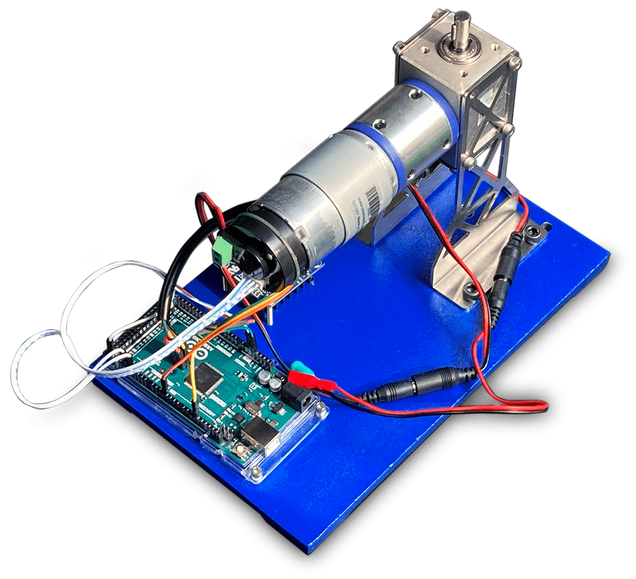
By the end of this article, you will be able to control a DC motor with a PID controller running on an Arduino:

If you are more of a visual learner, see the presentation slides.

motivation

Servo-motors (which are simply motors integrated with controllers and drivers) are significantly more expensive than the same actuators without a controller.

/*
Compare a linear actuator with a linear servo, or high-torque motor with a high-torque servo. Why such difference in price?
*/

Someone had to perform system identification, design a controller and a printed circuit board, wire up encoder(s) to read motor shaft position, integrate the motor driver, and design a housing that contains all these parts.

This self-contained package becomes their intellectual property that can be sold at a premium, unlike a commodity.

Sometimes it’s desirable to get a project off the ground quickly, but selling mass-produced robots means keeping production costs low to protect profits.

Robotics hobbyists will also find that they can stretch their budget much further for prototyping - and learn something in the process!

applications

While most of the world runs on PID controllers, they are often found in less-exciting roles: refrigerators, stoves, heaters, and inside industrial plants.

Do they really have a place at the forefront of robotics and automation? Let’s look at some use-cases.

personal robot

The PR2 (or Personal Robot) is the hardware the first version of Robot Operating System (ROS) was developed on.

With a mobile base, a pair of articulate arms, and a visual sensor array supplemented with laser scanning, it can perform many useful tasks:

The PR2 runs PI controllers on its motor control boards:

/*
Each motor/encoder on the PR2 has its dedicated Motor Controller Board (MCB). The MCB detects and counts transitions in the encoder signal, measures the motor current, and commands the voltage going to the motor. Each MCB runs a PI-control loop to control the motor current to a desired value, by commanding the motor voltage.
*/

retail robot

The Fetch robot is a mobile platform specifically designed for pick-and-place:

Fetch runs a variation of PID control on its motor control boards:

/*
Each motor has a dedicated motor controller board based on an STM32. This microcontroller runs a 17kHz effort controller on the brushless motor as well as realtime 1kHz PIV loops for velocity or position control […].
*/

inspection robot

The Anymal is a four-legged robot broadly useful for applications like warehouse inspections, rescue operations, security surveillance, forest and animal control, or teleoperation in hazardous environments:

Anymal is based on MIT Mini Cheetah, which runs a variation of PID control:

/*
Motor control, sensor measurement, and communication are handled by an STM32F446 microcontroller. […] An automatically tuned PI controller was used, which sets the gains of the current controller based on electrical parameters measured by the motor controller itself.
*/

alternatives

What about the highly dynamic robots that dominate today’s news? Are they also using PID controllers?

mpc control

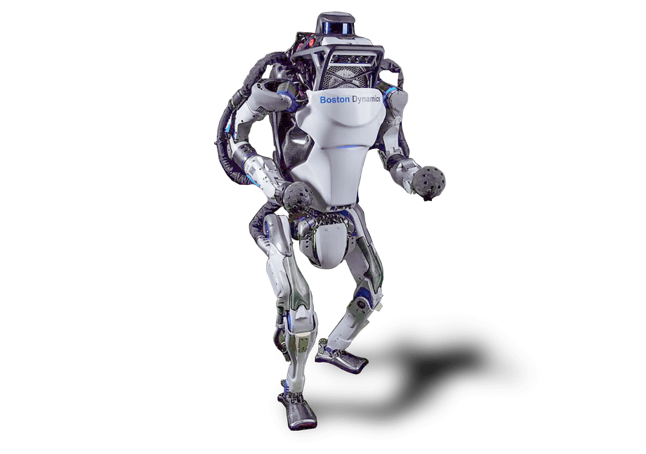
The Atlas series of robots from Boston Dynamics are using Model Predictive Control, or MPC for dynamic walking and balancing:

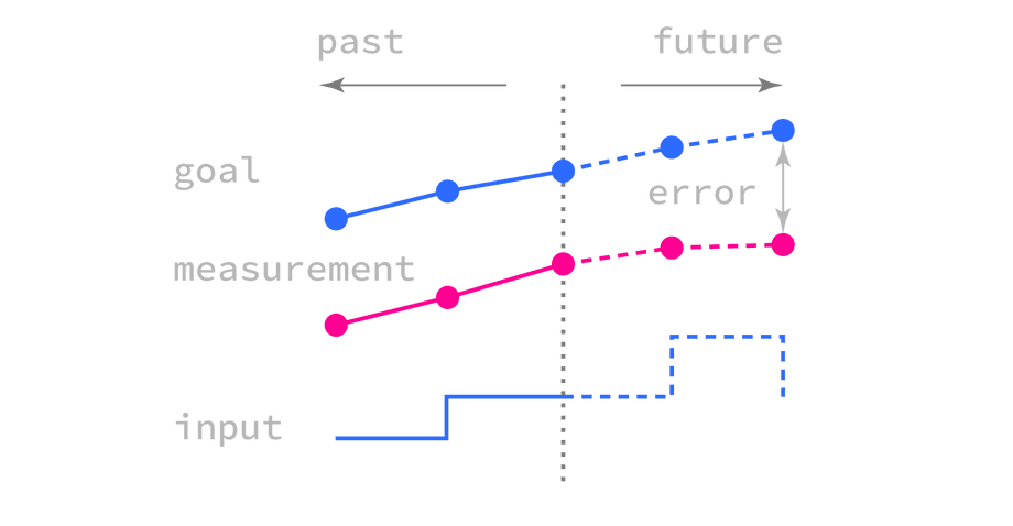
While PID controllers respond to changes without understanding the system they’re controlling, MPC controllers use a model similar to the Kalman Filter.

They run real-time physics simulation modeled by Lagrangian Mechanics to determine how to get the robot to the desired pose with the least effort.

non-linear control

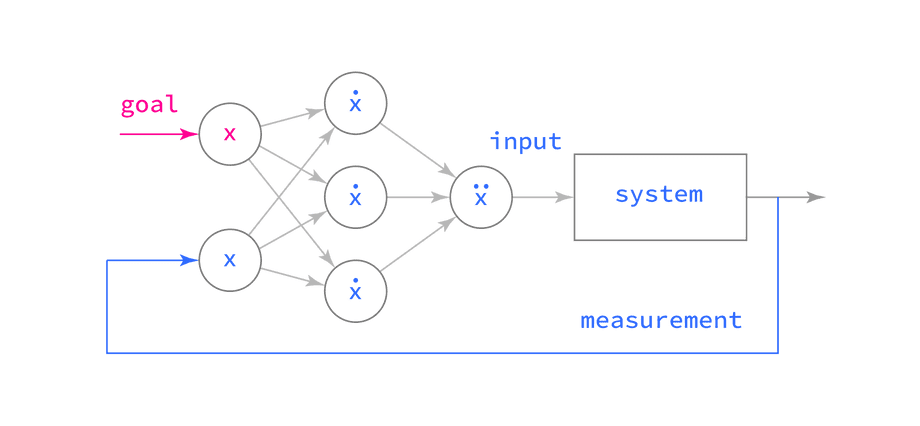
Non-linear controllers combine or replace PID with a neural network. Two notable companies using Machine Learning techniques to run the motors in their robots are Figure AI and Agility Robotics.

Figure 01 by Figure Robotics in California:

Digit by Agility Robotics in Oregon:

Non-linear controllers are able to learn the quirks of the physical systems they are controlling through reinforcement learning (RL) or convex gradient descent.

terms

The PID controller began its life as an electrical circuit designed by a Russian naval engineer, Nikolai Minorski, to automate ship steering. It was later adopted by the entrepreneur Elmer Sperry to create an autopilot for the U.S. Navy.

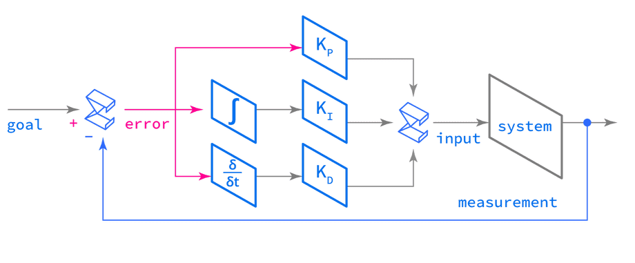
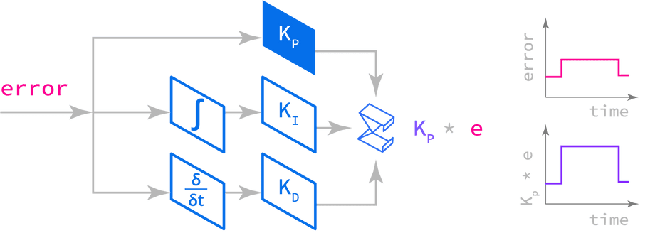
A PID controller is composed of three behaviors:

Proportional: attempts to close the distance to the goal
Integral: compensates for under-correcting in the past
Derivative: compensates for over-correcting in the future

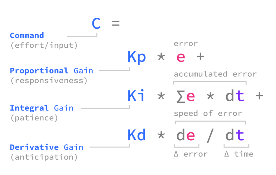
The Kp, Ki, and Kd weights applied to each term are called gains, and they are used to tune the overall behavior of the controller:

Proportional term: controls responsiveness and can be tuned for aggressive or laid-back behavior.
Integral term: controls disturbance rejection, and can be tuned to compensate for long-acting forces like wind, pressure, and gravity.
Derivative term: simulates friction, gradually “applying brakes” when in danger of over-correcting.

The three terms are simply summed together, which is represented by ∑ at the end of the diagram. This sum is called a command or an input.

what is an error?

The error in PID controller equations is the difference between the desired state and the measured state (the amount of mismatch to correct).

/*
For example, the desired temperature in a room versus the current temperature, or the desired servo position and its current position.
*/

The ∑ at the start of the diagram represents that the error is the goal (or setpoint) with the measurement subtracted from it.

proportional term

The proportional term reacts to the present error. How vigorously it reacts is configured by the proportional gain Kp.

A large proportional gain will result in more immediate and aggressive action, while a smaller gain will make the behavior more laid-back.

Selecting a proportional gain is about balancing the speed of response against the possibility of overshoot, or over-reacting.

integral term

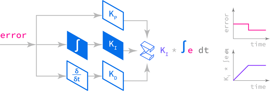
The integral term rejects constant disturbances: forces that are constantly pushing against the system.

The integral is multiplied by Ki, which acts as a weight that determines how much the controller should care about disturbance rejection.

This term was originally used to cancel out the effects of wind or currents in the high seas, since the controller must work consistently harder to defeat these forces when making its corrections.

Applied to robot actuators, it could be used to correct for gravity, such as when limbs are held out, under their own weight and the weight of held objects.

what is an integral?

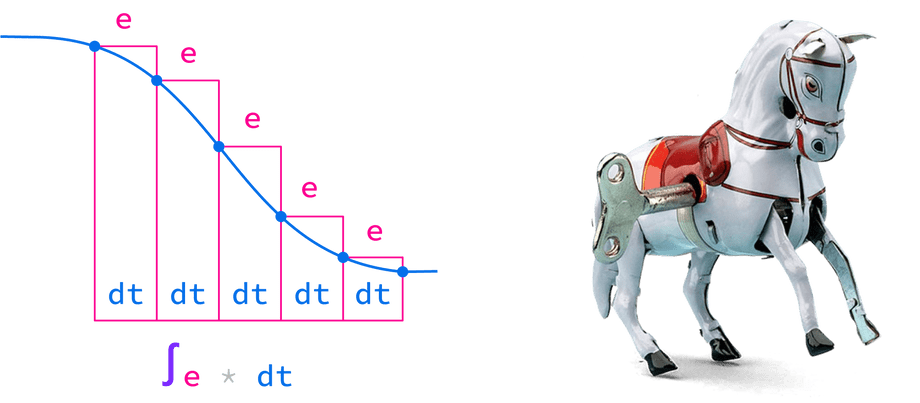
The name of this term comes from calculus: solving the same equation for multiple inputs in a row and summing the results.

For a PID controller, the integral term is the sum of all parts of error from beginning to now (and also the area under the graph of error over time):

The integral term accumulates error, winding up like a coiled spring that steadily pushes against any constant forces fighting the controller.

When the controller is “successful” (error is low) for an extended period of time, the tension “winds down” and the integral term stops acting.

derivative term

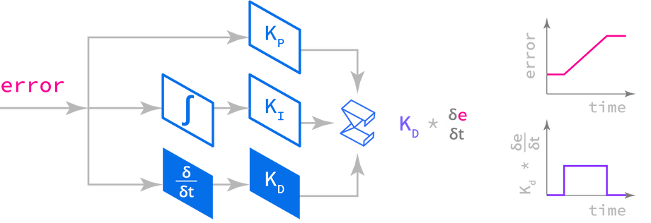
The derivative term applies brakes to control overshoot. The technical name used to describe braking action in mechanical engineering is “damping”.

The derivative is multiplied by Kd, which acts as a weight that determines how much the behavior of a PID controller is affected by damping.

Dividing the change in error by the change in time (time step) will get you the “speed” with which the error is changing, hence the equation for this term.

Since the amount of damping applied is proportional to speed, it can be also be thought of as synthetic, or simulated, friction which helps us tune the behavior of a controller in an intuitive manner.

what is a derivative?

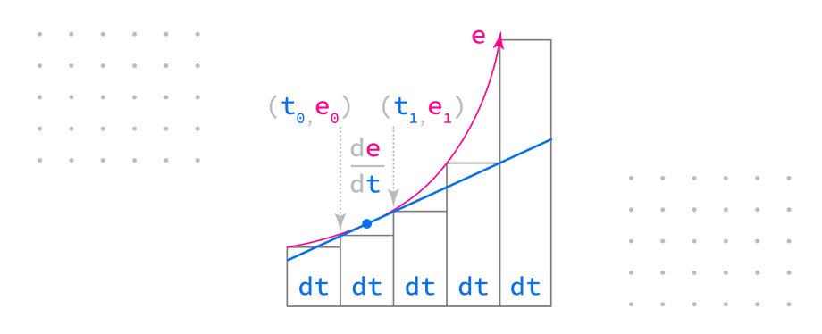
This term, originating from calculus, represents the slope of a curve at a specific point. When the error is plotted over time, it corresponds to the slope of the line between the previous and current error values:

Having made these two measurements we can “look ahead” and predict what the next value of error will be, so we can begin “pumping the brakes” ahead of time. The smaller the time step, the better the quality of predictions.

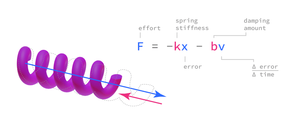
You may have noticed that PID equations bear resemblance to spring physics used to simulate ropes, cloth, and hair in video games:

Indeed, a PID controller is nothing more than a synthetic spring that “stretches” when the measurement is too far from the desired value, with “stiffness” defined by Kp and “damping” by Kd.

The Ki weight simulates a spring that “gets stiffer” the longer it’s stretched. This lets you tune the character of a controller by making it less “patient”, so it pushes harder when its efforts are unsuccessful and “relaxes” otherwise.

implementation

Let’s translate these equations into working C++ code:

float pid(
  float Kp,             // Proportional weight (responsiveness)
  float Ki,             // Integral weight (disturbance rejection)
  float Kd,             // Derivative weight (damping)
  float error,          // Measured vs Desired position
  float lastError,      // Error from last iteration
  float& integralError, // Accumulated error over all iterations
  float timeStep        // How much time passed
)
{
  // Integral equation
  integralError += error * timeStep;

  // Derivative equation
  derivativeError = (error - lastError) / timeStep;

  // Calculate the effort needed to reach desired position
  return (
    // Proportional term
    Kp * error +

    // Integral term
    Ki * integralError +

    // Derivative term
    Kd * derivativeError
  );
}

PID controllers run on a motor control board at a specific frequency (number of times per second) measured in (kilo)hertz. We can use an Arduino for this:

//
// Arduino Motor Control Board
//

#include <math.h>

// PID control parameters
const float FREQ_KHZ = 1.0;
const float KP = 1.0;
const float KI = 0.01;
const float KD = 0.01;
const float TOLERANCE = 0.01;
const unsigned long TS = (unsigned long)(1000.0f / FREQ_KHZ + 0.5f);

// PID control state
float goal = 0.0;
float lastError = 0.0;
unsigned long lastTime = 0;
unsigned long nextTime = 0;

void setup()
{
  Serial.begin(9600);
  lastTime = micros();
  nextTime = lastTime + TS;
}

void loop()
{
  // Scheduling
  unsigned long time = micros();

  if ((long)(nextTime - time) > 0) {
    delayMicroseconds((unsigned int)(nextTime - time));
  }

  time = micros();
  nextTime += TS;

  // Receive goal position
  if (Serial.available())
  {
    goal = Serial.parseFloat();
  }

  // Read encoder
  float measurement = readEncoder();

  // Calculate error
  float error = measurement - goal;

  // Calculate command
  if (fabsf(error) > TOLERANCE)
  {
    // Calculate time step (difference in microseconds to seconds)
    float timeStep = (float)(time - lastTime) * 1e-6f;

    // Calculate effort
    float command = pid(
      KP, KI, KD, error, lastError, integralError, timeStep);

    // Command motor velocity or torque
    writeMotor(command);
  }

  // Prepare for next loop
  lastTime = time;
  lastError = error;
}

The code needed to read the encoder position and communicate with the motor driver is application-specific, so it’s not included in the listing.

analysis

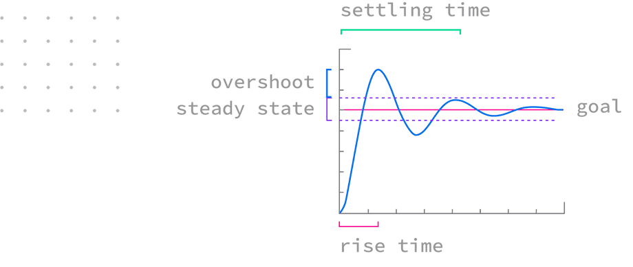
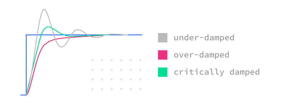
Controller behavior can be analyzed by plotting measurements from the point it starts acting on the error, until the error falls below threshold:

This envelope can help qualify the controller’s character:

Does the controller overshoot the goal position and by how much?
Does the controller get stuck in steady state, oscillating around the goal?
How fast does it respond (how long is the rise time)?
How fast does it stop acting (how long is the total settling time)?

Let’s add one component at a time to determine how they affect the envelope:

Only Proportional (P): may overshoot and oscillate around the goal without ever settling.
Proportional + Integral (PI): settles but may still overshoot.
Proportional + Integral + Derivative (PID): minimizes overshoot, settling as quickly as possible.

Tuning a PID controller is about balancing responsiveness against overshoot and steady state error. This balance is usually described as:

Under-damped: the controller is too aggressive, regularly missing and having to backtrack.
Critically damped: the controller is balanced, with minimum overshoot, rise time, and no steady state oscillation.
Over-damped: the controller is too laid-back and slow.

troubleshooting

As seen before, the integral term acts like a coiled spring: the longer it takes for the controller to reach its goal, the more tightly it’s wound up.

This makes the controller “live in the past” for a while, unable to adjust to its new reality and reacting longer than necessary:

Fortunately there is a simple solution to windup: clamping the integral gain by introducing two more parameters: Imin and Imax:

integralError = clamp(integralError, Imin, Imax);

Another common issue is steady state error: when the controller endlessly hovers around the goal, missing it over and over again by a small amount:

This behavior can be fixed by increasing integral gain or introducing a tolerance below which the error is ignored and the controller stops acting:

if (abs(error) > TOLERANCE)
{
  // run PID controller
}
else
{
  // don't run PID controller
}

A controller can also begin to oscillate when there’s a delay between the controller acting and seeing the results of its actions:

This will causes a controller to over-compensate because it thinks the effort its applying is not working. To fix issues caused by delay:

Lower the proportional gain
Lower disable the integral gain
Move the controller closer to feedback
Bake the sample delay into the model used to tune the controller

PID controllers can also suffer from instability, manifesting as violent oscillations that gradually increase in amplitude:

This could be caused by gains that are set too high, a time step that is too coarse, or a high sample delay.

tuning

Plugging in PID gains manually is like tuning a guitar without a tuner: it’s easy to get something that’s good enough, but never perfect:

Start with Kp 10, Ki 1, Kd 1 and watch the behavior.
If the controller reacts very aggressively, scale the terms down by 10.
If the controller reacts too slowly, scale the terms up by 10.
Add or subtract small amounts to each of the three terms.
Try setting various terms to 0 to turn them off.

In this section we’ll explore using Matlab System Identification Toolbox to estimate a mathematical model for the system being controlled, and Control System Toolbox to tune a PID controller automatically.

/*
Why use Matlab? Precise PID tuning requires advanced techniques like identifying an Autoregressive Exogenous model, and calculating PID gains using Frequency Response analysis. Using wizards will let us get immediate gratification and postpone treating these topics until later!
*/

system identification

System identification is a process used to estimate a mathematical model of the control system. This captures how the measurements from the encoder change when velocity or torque commands are sent to the motor.

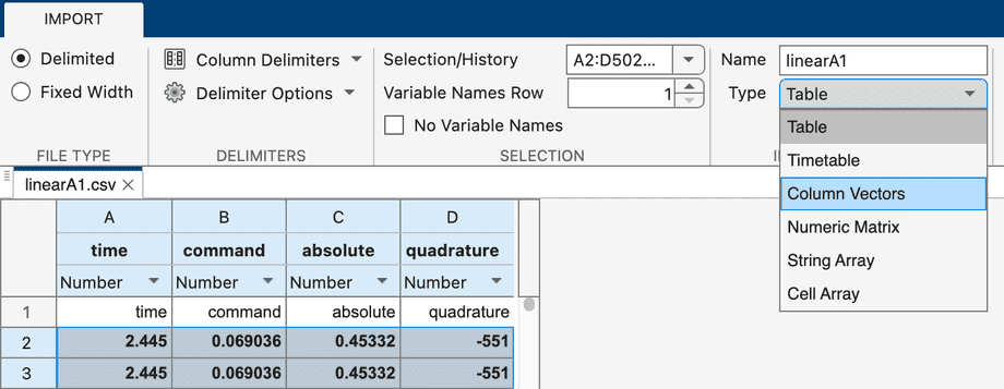
To perform system identification, we need a dataset that consists of time, commands, and measurement samples:

The time column records the current time, usually in seconds as a decimal number, to allow for microsecond accuracy.
The command column records the command sent to the motor. This can be normalized to -1...1 range (maximum effort in forward and reverse directions, with 0 signifying a complete stop).
The measurement column contains the encoder reading recorded at the same time. This can also be normalized to 0...1 range between the minimum and maximum achievable absolute position, or left as an integer when using a quadrature encoder.

I built a PID Tuner Web App utility to facilitate recording these samples and simplify experimentation by plugging in different PID gains:

Begin by preparing the hardware (a motor tuning fixture):

Connect an Arduino board to motor driver, encoder, and your computer.
Connect a power supply and a motor to the motor driver.

Record a step response:

Clone the PID Tuner Web App repository and follow the setup guide.
The web app uses Robot Operating System (ROS) to talk to an Arduino. ROS only works on Linux, but you can use Multipass to spin up an Ubuntu 20.04 VM on Mac and Windows.
The Arduino code in this project can be customized to integrate different encoders and motor drivers if necessary.
Draw a pattern in the Step pane, making the motor spin forward and backward with different velocities:
Click play to play back the pattern, sending these commands to the motor and recording encoder measurements.
Click the export button to download the CSV dataset.

Install auto-tuning tools:

Import the dataset:

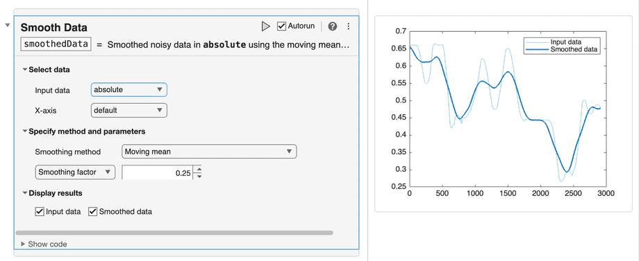
Click Import Data on the Home tab in Matlab:
Select the columns, and choose to import as column vectors:

Smooth the imported data:

On the Home tab in Matlab, click New, then select Live Script:
When the new live script opens, and click Task on the Home tab, then select Smooth Data:
In the Smooth Data widget that gets placed, pick your encoder column as the Input data, and Gaussian as the Smoothing method:
This will automatically create a column vector called smoothedData as a global variable, and even display a before/after chart. The live script can be closed without saving changes.

Perform system identification:

Click System Identification on Apps toolbar in Matlab:
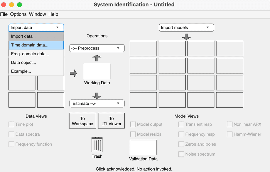
Click Import data dropdown and select Time domain data…:
In the Import Data dialog that opens, type in the names of the workspace variables corresponding to the imported column vectors:
- Input is the name of the column with motor commands.
- Output is the name of the column with encoder readings. Use smoothedData here.
- Sample time can be calculated by looking at the average difference between time samples in the imported dataset.
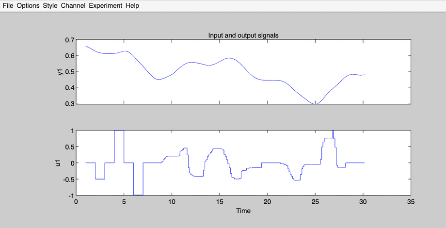
Click Time plot to preview imported (correlated) data:
Click Estimate dropdown and select Transfer function models….
On the Estimate Transfer Functions dialog, select Discrete-time.
Delay options can be configured under Delay accordion.
Click Estimate, and the resulting model will be placed in one of the empty slots in System Identification dialog.
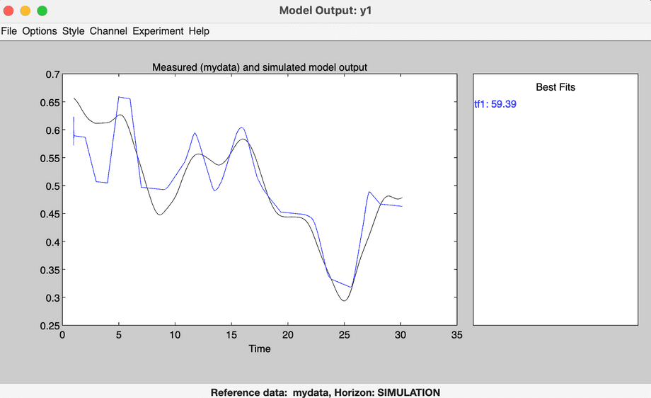
With the identified model selected (selection is communicated through increased line thickness in the preview slot), click Model output to see a preview of how the model fits over the original measurements:
This process can be repeated, filling in empty slots with models identified by using different settings. Model Output will then preview all of the models against the original data.
Drag the best model to the To Workspace button above the Trash icon to save it into a global variable for the next step.

auto-tuning

We can tune the PID controller by using the identified model:

Click PID Tuner on Apps toolbar in Matlab:
Import the plant identified and saved in the previous section:
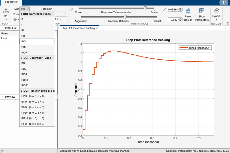
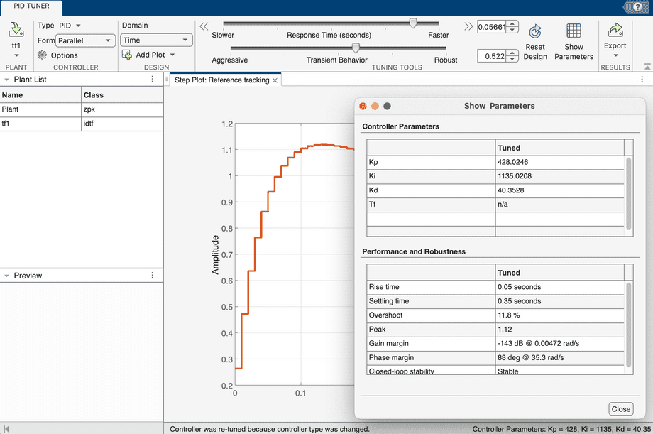
Change the controller Type in the dropdown, and use the sliders to set the requirements for the controller performance:
Click Show Parameters to see the suggested PID gains, which are also displayed in the status bar at the bottom:
Plug in the suggested PID gains, move the position slider in PID Tuner web app, and watch how the motor responds!

PID Controlcopy link

overviewcopy link

motivationcopy link

applicationscopy link

personal robotcopy link

retail robotcopy link

inspection robotcopy link

alternativescopy link

mpc controlcopy link

non-linear controlcopy link

termscopy link

what is an error?copy link

proportional termcopy link

integral termcopy link

what is an integral?copy link

derivative termcopy link

what is a derivative?copy link

implementationcopy link

analysiscopy link

troubleshootingcopy link

tuningcopy link

system identificationcopy link

auto-tuningcopy link